A Diffusion-Driven Fine-Grained Nodule Synthesis Framework for Enhanced Lung Nodule Detection from Chest Radiographs
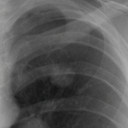
Ours (diffusion)
Realistic nodules, with control over what they look like
Detecting lung nodules on chest X-rays is hard, partly because detectors don't see enough examples of every kind of nodule. We train a diffusion model that paints a nodule into any chosen spot of a real X-ray, and lets you choose its shape and size (through a mask), its border, its texture, whether it is calcified, and how subtle it is.
Each characteristic is learned by its own small add-on module (a LoRA adapter). To combine two characteristics in one nodule, we train the adapters with an extra loss that keeps them from interfering with each other. Adding the generated nodules to a detector's training data improves detection on in-house and public test sets.
What each characteristic looks like, and how well it works
Radiologists describe a nodule by a few traits that matter for diagnosis. Pick one to see its definition, examples generated by our model, and the numbers for that trait. Click any image to enlarge it.
How it works
The model is trained in three stages. The first two teach it to draw realistic nodules where a mask says; the third adds control over individual characteristics. Click a stage.
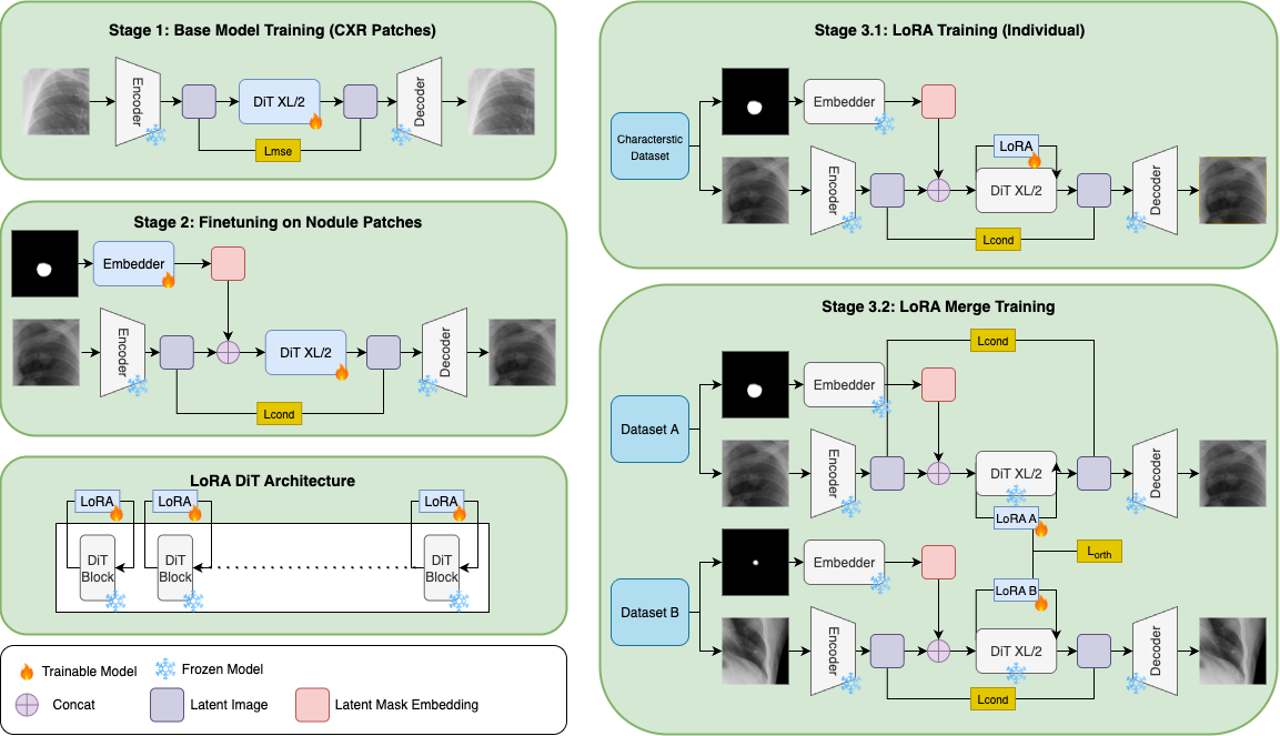
From a mask to a nodule
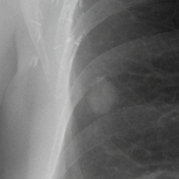
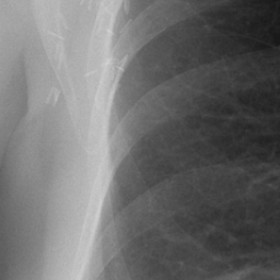
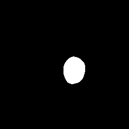
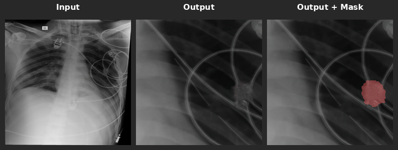
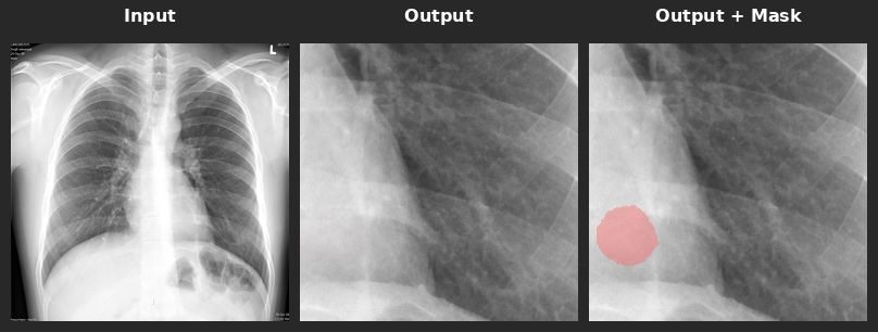
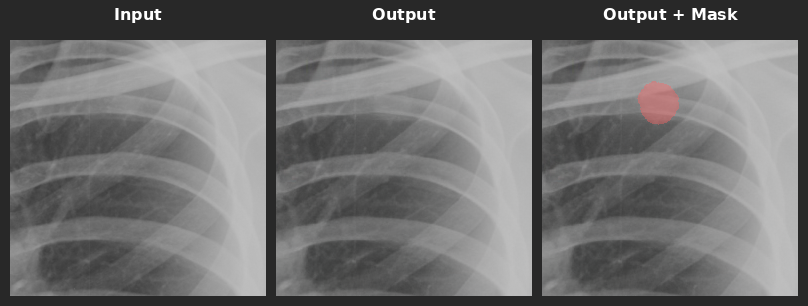
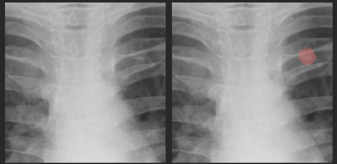
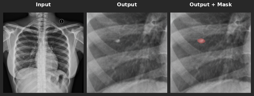
At test time you give the model an X-ray patch and a binary mask. It fills the masked region with a nodule of that shape and size and leaves the surrounding lung untouched. Drag the slider to compare the input and the output.
Why separate adapters instead of one conditioning signal
A natural idea is to feed the characteristic label into the model with classifier-free guidance (CFG), the same way the mask is fed in. In practice, guiding on both the mask and the labels made them compete and blurred the nodule's boundary. So the mask keeps CFG, and each characteristic gets its own LoRA adapter. The adapters follow their characteristic much more closely (lower FID is better):
A LoRA adapter freezes the model's weights \(W_0\) and learns a small low-rank update \(\Delta W = AB\) (rank 32 here). Each adapter adds about 6.2M parameters, under 1% of the frozen model, and sits in the attention layers of all 28 transformer blocks.
A slider for how hard a nodule is to see
Radiologists graded each training nodule from 1 (most subtle) to 5 (most obvious). Rather than training one adapter per grade, we tie the grade to the adapter's strength \(\alpha\): subtle nodules are trained with a small \(\alpha\) and obvious ones with a large \(\alpha\),
At generation time, turning \(\alpha\) down makes the same nodule fainter. Try it on one mask:
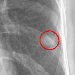
Radiologists were shown sets of three such versions and asked to order them from most obvious to most subtle. The panel's majority order matched ours in 80% of sets. Subtle nodules also helped the detector most where it was weakest; see the subtle-nodule results.
Combining adapters without interference
Real nodules rarely have just one trait. A benign nodule is often calcified and smooth; a worrying one is often irregular and uneven in texture. So we want to switch on two adapters at the same time.
Problem 1: they fight over the same pixels
In natural images, a "style" adapter and an "object" adapter usually act on different parts of the image. Here every adapter acts on the same small nodule region, so their updates compete. One trait tends to dominate, and artifacts appear near the mask edge.Problem 2: their updates overlap
Adapters trained separately end up pointing in similar directions in weight space. Most of an adapter's weights are near zero (60–70% below 0.01), so the few that matter collide when you average two adapters. This hurts every merging method we tried: linear merging, switching and ZipLoRA.Our fix is to train the two adapters together and add a penalty whenever their updates overlap:
The penalty is zero when the two updates are orthogonal, meaning they change the model along independent directions. With it, simply averaging the adapters works, and each trait stays adjustable through its own \(\alpha\).
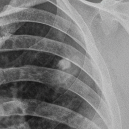
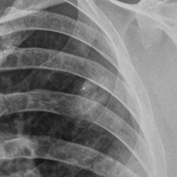
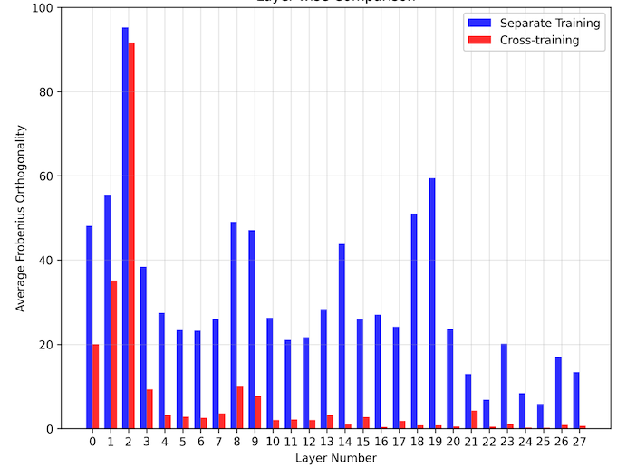
A fair worry is that the loss just shrinks the adapters toward zero, which would also make the overlap small. It doesn't: the jointly trained adapters actually have larger weights than separately trained ones, so the loss is separating their directions rather than switching them off.
Does it help?
We check three things: whether radiologists find the nodules realistic and correctly characterised, whether the nodules improve a detector, and how the model compares with other nodule generators.
Three experienced radiologists took three blinded tests. Results can be counted two ways: majority vote (the panel's decision per image) or pooled (every individual answer counted). Whiskers show 95% confidence intervals.
A detector (Swin-Tiny encoder with a U-Net++ head) is trained on 10k real nodules and about 100k normal X-rays, plus a growing number of generated nodules. Performance is measured on three test sets.
All generators were trained on the same in-house data. We compare two GANs (ACGAN, ReACGAN) and CR-Fill, the best inpainting method in the NODE21 generation challenge.
A classifier with one output per characteristic is trained on 5k real nodules, then again with about 400 generated nodules per characteristic (2k in total) added. Segmentation IoU on the in-house test set:
JSRT grades its nodules from S1 (most subtle) to S5 (most obvious). We add 12k subtle nodules from the subtlety slider (\(\alpha < 24\)) to training and measure classification accuracy at each grade.
Datasets
The in-house data has 1.2M frontal chest X-rays from partner hospitals, about 40k of them with nodules. Every nodule has a shape outline and characteristic labels from three experienced radiologists. JSRT and ChestX-ray14 are public test sets; their nodule boxes were refined into outlines with our segmentation model and checked by radiologists.
| Diffusion train | Detector train | In-house test | JSRT test | ChestX-ray14 test | |
|---|---|---|---|---|---|
| All X-rays | 1,100,000 | 100,000 | 12,000 | 247 | 500 |
| With nodules | 28,000 | 10,000 | 2,000 | 154 | 66 |
Compute
- Backbone: DiT-XL/2 (about 680M parameters, 28 transformer blocks) on 256×256 patches, encoded to 32×32 latents. Stage 1 took about a week and Stage 2 about two days, each on four NVIDIA L40 GPUs.
- Adapters: about 10 hours per characteristic on four L40s; 20–30 hours for a jointly trained pair.
- Generation: 250 DDIM steps, about 10 seconds per nodule.
Limitations
Some combinations of adapters produce nodules outside what the model saw in training. We evaluate pairs of characteristics only. The loss extends to three or more adapters by penalising every pair, but the data has too few nodules labelled with several traits at once for a fair test, and many three-way combinations are rare in practice.
BibTeX
@inproceedings{goyal2026nodule,
  title     = {A Diffusion-Driven Fine-Grained Nodule Synthesis Framework
               for Enhanced Lung Nodule Detection from Chest Radiographs},
  author    = {Goyal, Aryan and Singh, Shreshtha and Mittal, Ashish and
               Tadepalli, Manoj and Kumar, Piyush and Putha, Preetham},
  booktitle = {Medical Imaging with Deep Learning (MIDL)},
  year      = {2026},
  url       = {https://arxiv.org/abs/2603.01659}
}