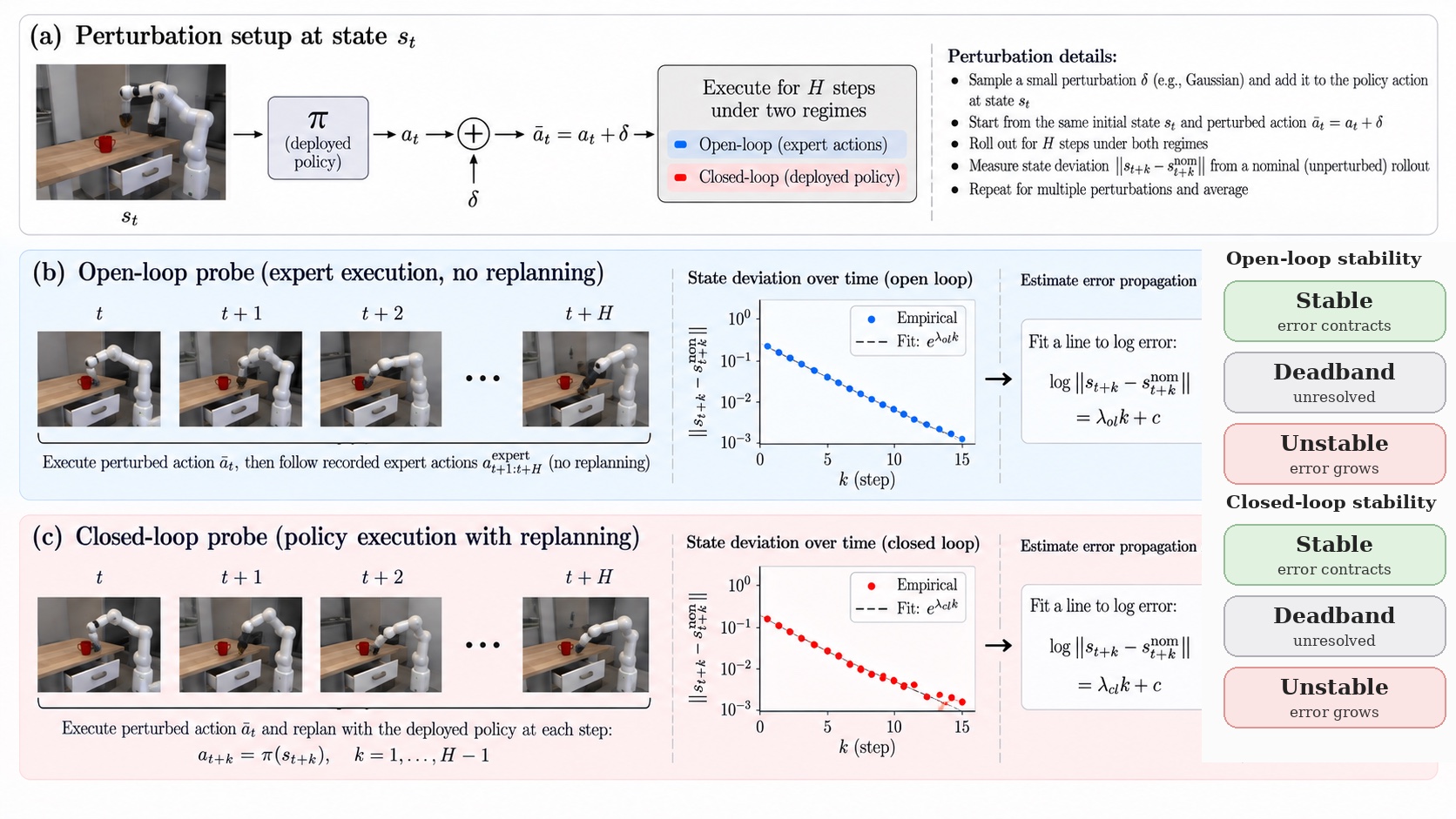
Action chunking improves the performance of policies learned by behavioural cloning, and several mechanisms have been proposed to explain why, including temporal consistency, horizon reduction, representation learning, and reduced error compounding. Every one concerns the error the policy introduces, whether by reducing how much of it enters or how often it re-enters the policy's own input. We instead study what happens to an action error once it enters the system. At each state, we inject a small action error and measure how fast it grows or shrinks under two execution regimes: open-loop, where the rest of the chunk is replayed without replanning, and closed-loop, where the policy replans after the perturbation. The fitted rate labels each state as contracting, expanding, or unresolved. Across twelve manipulation tasks from three benchmark suites, we find that confidently stable states are rare, while error amplification is common among states whose propagation rate can be resolved. We further find that the measured propagation rate depends strongly on the fitting horizon: amplification is typically front-loaded, so short windows can substantially overestimate longer-horizon propagation. Finally, we train predictors on these labels and find that a state's open-loop regime can be recovered from camera frames and proprioception alone, without a simulator, while its closed-loop propagation is only partially recoverable because it also depends on how the policy acts after the perturbation. These results suggest that error-compounding arguments alone do not provide a complete account of action chunking: neither passive open-loop dynamics nor policy replanning consistently contracts an injected error, and replanning rarely turns open-loop amplification into confident contraction. This also suggests that closed-loop reactivity should be trained explicitly, using perturbation- and tree-coverage-oriented training to expose the policy to deviations it must recover from, rather than expected to emerge reliably from standard imitation learning.
Background
Imitation-learned manipulation policies increasingly predict chunks of actions rather than single steps. A chunked executor plays \(k\) actions open-loop and then replans, and \(k\) is chosen once per task. Chunked execution is widely reported to outperform single-step execution, but the explanation is contested. The accounts on offer attribute the gain to different mechanisms:
Every one of these accounts concerns the error that enters the loop: how often the policy introduces one, or how large it is when introduced. None of them addresses what happens to the error afterwards, whether the dynamics contract it or expand it, and small deviations are inevitable in learned policies.
The theory
The theoretical bounds do speak to what happens after an error enters, but they assume a single global contraction rate for the dynamics rather than a rate that varies with state. Zhang et al. (2025) assume the true dynamics are open-loop exponentially incrementally input-to-state stable with a fixed decay factor \(\rho\in(0,1)\): roughly, \(\rho\) determines how quickly a deviation between trajectories decays from one step to the next. Under this assumption they show that sufficiently long action chunks restore exponential stability of the learned closed loop, with the required chunk length
\[k \;\ge\; k^{\star} \;=\; \log(1/\rho)^{-1}\,\log\!\big(\mathrm{poly}(L, C_{\mathrm{ISS}})\big),\]
so weaker contraction (larger \(\rho\)) requires longer chunks. Lazzati et al. (2026) likewise derive their bound under deterministic Lipschitz dynamics. In both analyses the relevant dynamical constants are assumed rather than measured and treated as global. A manipulator in free space and the same manipulator during contact need not propagate an error at the same rate.
Replanning is the other way an error can be dealt with, and it raises the same question about the deployed policy rather than the plant. The expert paired with the true dynamics, \((\pi^{\star}, f)\), is stable by construction, since a human demonstrator sees the error and corrects it. What matters at deployment is the learned policy paired with the same dynamics, \((\hat{\pi}, f)\), and stability of the former does not imply stability of the latter. Whether \((\hat{\pi}, f)\) is stable at a given state is an empirical property of the trained policy in its environment, to be measured rather than inherited from the demonstrator.
Our framework
The idea is a small experiment repeated at many states. Pick a state, nudge the first action a little, and watch how far the robot drifts from where it would have gone without the nudge. If the gap shrinks over the next few steps, that state is stable; if it grows, it is unstable.
The open-loop probe is run at three kinds of states, and the closed-loop probe at the policy's own replan points, so the two regimes can be compared at identical states.
| Stamp type | State from | Actions used | \(K\) |
|---|---|---|---|
| demonstration | demonstration file | demonstrator actions, as recorded | 24 |
| rollout | policy rollout | policy actions, as recorded | 24 |
| policy chunk | policy rollout, at a replan boundary | chunk emitted by the policy | 8 or 24 |
| closed loop | policy rollout, at a replan boundary | policy replans at every step | 24 |
Demonstration versus rollout changes the state distribution; rollout versus policy chunk changes the action source. For policy-chunk stamps, \(K\) is capped by the emitted chunk length: 8 actions for the diffusion policies and up to 24 on RoboCasa.
We label twelve tasks across three benchmark families: robomimic
(lift, can, square, tool_hang, per-task
diffusion policies), MimicGen (coffee,
nut_assembly, square_d0, stack_d0), and
RoboCasa (OpenCabinet, OpenDrawer,
PickPlaceCounterToCabinet, TurnOnSinkFaucet, driven by the public
GR00T N1.5 checkpoint).
Results
Open-loop. Across all three stamp types, unstable states are more common than stable states among measurements that clear the gates, while most stamps fall in the deadband. The deadband is not noise: 90–99% of stamps that clear Gate 1 also clear Gate 2 at \(K{=}24\). It is driven by rates too small to cross the amplification threshold; on lift, 78% of demonstration stamps have \(|\lambda| < 0.0289\). Within robomimic the median rate rises from can (\(0.009\)) to lift (\(0.015\)), square (\(0.017\)), and tool hang (\(0.026\)), the most precision-demanding task. Rollout medians stay close to their demonstration counterparts (lift \(0.019\) vs. \(0.015\)), so moving from expert states to policy-visited states does not substantially change how the plant propagates a small error.
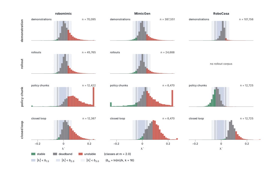
The error is front-loaded. The perturbed branches separate rapidly in the first few steps and then flatten rather than keep growing at the same rate. The measured rate therefore depends on the fitting window: a short window fits the initial rise and reports more unstable states, a long window averages that rise with the plateau and pulls \(\lambda\) toward zero. \(\lambda\) is a summary of propagation over an interval, not a time-invariant rate for the whole trajectory, and a short chunk can end while the error is still growing where a longer one continues through the plateau.
Closed-loop. Closed-loop stability is substantially rarer than passive contraction under the same measurement: at \(m{=}2\) the stable class holds only 3–88 stamps per task, despite hundreds of non-stable stamps. Comparing the two regimes at the same policy-replan states, the [OL unstable, CL stable] cell is near zero on all three benchmark families. States that amplify an error in open loop rarely contract it when the policy replans; they move to the deadband or remain unstable. Replanning trades away the temporal commitment of a chunk for reactivity without reliably reducing error propagation.
This exposes a gap in standard imitation training. The policies are trained directly from expert demonstrations, without perturbation augmentation or recovery supervision, which constrains them on the demonstrated states and says little about recovery after a deviation. Closed-loop contraction may need to be encouraged explicitly by training on perturbed states and their recovery actions, in the spirit of DART (Laskey et al., 2017) and Simchowitz et al. (2025).
Prediction
The open-loop rate is a property of the state the robot is in, so we ask whether it is visible. A frozen V-JEPA 2 ViT-L encoder over a short window of camera frames, with proprioception over the same window, feeds a two-layer head that predicts \(\lambda\) and a logit for the unstable class. P receives frames and proprioception only; A1 additionally receives the action chunk under evaluation. Classification uses only stamps that clear both gates; regression uses all stamps.
Open-loop is visible. On demonstration and rollout stamps the predictor
reaches AUROC between \(0.63\) and \(0.94\) where the negative class is sufficiently
supported, strongest on tool_hang and mg-coffee. Regression is
weaker, recovering a tenth to a quarter of the constant-median error: the model is better
at identifying which states are prone to amplification than at predicting how much the
error will amplify. Adding the action sequence improves regression and rank correlation,
as expected when the target depends on the sequence replayed.
Closed-loop is only partly recoverable. With the same predictor, inputs, and stamps, switching the target to the closed-loop rate still improves on the constant-median baseline on most regression cells, and AUROC exceeds \(0.70\) in half of the cells with both classes present, but the gains are less uniform. The closed-loop rate depends not only on the configuration but on how the policy acts after the perturbation.
| Dataset | Input | Open-loop target | Closed-loop target | ||||
|---|---|---|---|---|---|---|---|
| MAE0 | MAE | \(\rho\) | MAE0 | MAE | \(\rho\) | ||
| lift | P | .0792 | .0535 | .757 | .0322 | .0178 | .819 |
| lift | A1 | .0792 | .0400 | .795 | .0322 | .0164 | .841 |
| can | P | .0981 | .0635 | .706 | .0395 | .0323 | .520 |
| can | A1 | .0981 | .0568 | .762 | .0395 | .0305 | .553 |
| square | P | .0877 | .0790 | .510 | .0370 | .0364 | .332 |
| square | A1 | .0877 | .0742 | .560 | .0370 | .0357 | .386 |
| tool_hang | P | .0887 | .0687 | .627 | .0377 | .0393 | .239 |
| tool_hang | A1 | .0887 | .0664 | .637 | .0377 | .0347 | .333 |
| mg-coffee | P | .0833 | .0842 | .149 | .0400 | .0311 | .436 |
| mg-coffee | A1 | .0833 | .0835 | .215 | .0400 | .0317 | .455 |
| mg-nut | P | .0959 | .0941 | .284 | .0391 | .0373 | .374 |
| mg-nut | A1 | .0959 | .0927 | .324 | .0391 | .0344 | .474 |
Prediction of open- and closed-loop propagation rates at the same policy-replan stamps. Both heads use the same trunk and inputs; only the target differs. \(\mathrm{MAE}_0\) is the constant-median baseline, \(\rho\) is Spearman correlation with the measured rate. Bold denotes improvement over the baseline.
Conclusion
We studied what happens after an action error enters a chunked imitation-learning system, rather than how often the policy introduces one. Confidently stable states are uncommon, amplification is common among states whose rate is resolved, and replanning frequently removes confident amplification but rarely produces confident contraction. Propagation is strongly state- and horizon-dependent: even within a single task, rates vary substantially across states, so the assumption of a single global contraction rate is not supported empirically even at the task level, let alone across a benchmark.
These results do not determine the best execution horizon by themselves; stability is one factor alongside task performance, temporal consistency, and replanning cost. They do suggest that closed-loop error recovery should not be expected to emerge reliably from standard imitation learning. If it is desired, it should be trained explicitly, by exposing the policy to perturbations and recovery trajectories through perturbation- and tree-coverage-oriented training.
Label videos
Each clip starts at one labeled state: the moment we nudge the first action. From there it plays the next \(K{=}24\) time steps, which is the whole window the label is measured over, so the clips are short by design. The white path is the robot's end-effector when nothing is nudged; the coloured paths are the \(N{=}8\) nudged copies. Watch whether the coloured paths pull back toward the white one (stable), fan out away from it (unstable), or neither (deadband). The label and its rate are printed in the corner.
Demonstration stamps, \(K{=}24\), \(m{=}2.0\). Buttons 1–2: unstable, highest \(\bar{\lambda}\) clearing both gates. 3–4: deadband, \(\bar{\lambda}\) nearest zero. 5–6: stable, most negative \(\bar{\lambda}\) clearing both gates. Hover a button for the stamp.
@misc{goyal2026stability,
  title         = {Measuring the Stability Assumption Behind Action Chunking},
  author        = {Goyal, Aryan},
  year          = {2026},
  eprint        = {2610.01626},
  archivePrefix = {arXiv},
  url           = {https://arxiv.org/abs/2610.01626},
}