Robot Learning: A Mathematical Guide to Training Policies (in progress work)
In this walkthrough
The setup
$x_t\in\mathbb{R}^d$ is the robot’s state, and $t$ is the time step. For a robot arm, the state may include joint angles and velocities. $u_t\in\mathcal{U}\subseteq\mathbb{R}^m$ is its action, such as a joint velocity command. An episode lasts $T$ steps.
The dynamics $F$ determine the next state from the current state and action:
\[x_{t+1}=F(x_t,u_t).\]We assume deterministic dynamics: the same state and action always give the same next state.
The robot receives an observation $o_t=G(x_t)$. This may be the full state, a camera image, or sensor readings. A policy $\pi$ uses this observation to choose an action. A deterministic policy gives one action; a stochastic policy gives a distribution from which an action is sampled. We write $\pi(x)$ as shorthand for $\pi(G(x))$.
$\pi^\star$ is the expert policy that provides demonstrations, and $\hat\pi$ is the learned policy. The expert need not be optimal. Starting from the same initial state, they generate two sequences of states and actions, called trajectories:
\[\begin{aligned} \text{Expert: }&(x_1^\star,u_1^\star),(x_2^\star,u_2^\star),\ldots\\ \text{Learner: }&(\hat x_1,\hat u_1),(\hat x_2,\hat u_2),\ldots \end{aligned}\]$d_\pi^t$ is the state distribution at time $t$ under policy $\pi$: it describes which states the robot is likely to occupy at that step across repeated episodes. The initial state, and any sampled actions, can vary between episodes. We compare the expert and learner using the same initial-state distribution.
The average state distribution over all $T$ steps is
\[d_\pi=\frac{1}{T}\sum_{t=1}^{T}d_\pi^t.\]Equivalently, run the policy, choose one of the $T$ time steps uniformly at random, and look at the state there. Its distribution is $d_\pi$.
Demonstrations contain states visited by the expert, described by $d_{\pi^\star}$. At deployment, the learner visits states described by $d_{\hat\pi}$. These distributions can differ:
\[\boxed{d_{\hat\pi}\neq d_{\pi^\star}\quad\text{in general}}.\]A different action can move the learner to a state poorly covered by the demonstrations. Its next action is then chosen from that new state, so further errors can carry it farther from the expert’s trajectory. This is the distribution shift illustrated below.
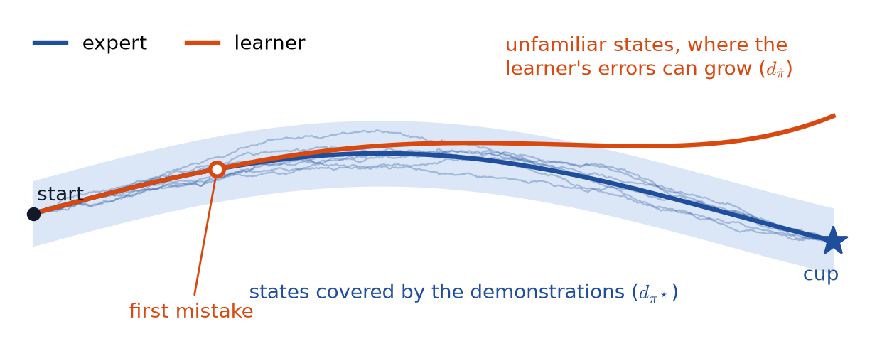
The dynamics have not changed; the learner’s actions change the states it visits. This is the distinction from ordinary supervised learning emphasized by Ross and Bagnell (2010).
Takeaway. Demonstrations are drawn from $d_{\pi^\star}$, but the robot is evaluated on $d_{\hat\pi}$, and the policy itself creates the gap between the two. This is what separates imitation learning from ordinary supervised learning.
How far did the rollout drift?
To reason about this gap, we first need a way to say how much worse the learner is than the expert. The most direct option is to run both from the same start and compare their trajectories step by step. Is trajectory distance the right yardstick?
At each timestep, compare the two states and the two actions, and add up the result:
\[\boxed{ J_{\mathrm{Traj},T}(\hat\pi)=\mathbb{E}_{\hat\pi,\pi^\star}\!\left[\sum_{t=1}^{T}\min\left\{1,\,\|\hat x_t-x_t^\star\|_2^2+\|\hat u_t-u_t^\star\|_2^2\right\}\right] }.\]The state term $\lVert\hat x_t-x_t^\star\rVert_2^2$ measures how far the learner has drifted from the demonstrated state, and the action term $\lVert\hat u_t-u_t^\star\rVert_2^2$ measures how different its command is. The minimum caps each timestep’s contribution at $1$, so a single wild step cannot dominate the sum. The expectation averages over randomness in the initial conditions and the policies, when present. Because of the cap,
\[0\leq J_{\mathrm{Traj},T}(\hat\pi)\leq T.\]This number measures mismatch, not success. A learner can take a different path to the cup and still grasp it, and trajectory distance counts that as error. Or it can track the expert closely for 95 of 100 steps and knock the cup over in the last five, and trajectory distance charges it little more than $5$ out of a possible $100$, even though the task failed. To judge the task, we need the task’s own cost.
Takeaway. Trajectory distance tells us how different the learner is from the expert, not how well it does the task. The two quantities we actually need come next: the cost we care about, and the error we can measure.
What we care about, and what we can measure
Two quantities run through the rest of this post. The first is what we care about: how much worse the learner does at the actual task. The second is what we can compute from demonstrations: how well the learner predicts the expert’s actions. Every result that follows is a bridge from the second to the first. What exactly sits at the two ends of that bridge?
What we care about. Let $c_t(x_t,u_t)\in[0,1]$ be the cost at timestep $t$, with smaller values meaning better performance. The expected cumulative cost of a policy $\pi$ is
\[J(\pi)=\mathbb{E}_{\tau\sim\pi}\!\left[\sum_{t=1}^{T}c_t(x_t,u_t)\right],\]where the expectation is over trajectories $\tau$ generated by running $\pi$, including the initial state and any randomness in the policy. Since each step costs at most $1$, we have $0\leq J(\pi)\leq T$. The quantity we want to control is the extra cost the learner pays over the expert when both are deployed, which we will call the deployment gap:
\[\boxed{R_{\mathrm{cost}}(\hat\pi;\pi^\star)=J(\hat\pi)-J(\pi^\star)}.\]What we can measure. Demonstrations give us expert states paired with expert actions, so we can measure how far the learner’s actions are from the expert’s on those states. With $u_t^\star=\pi^\star(x_t)$ and $\hat u_t$ sampled from the learner at the same state,
\[\boxed{ R_{\mathrm{expert},L_p}(\hat\pi) =\sum_{t=1}^{T}\mathbb{E}_{x_t\sim d_{\pi^\star}^t}\!\left[\mathbb{E}_{\hat u_t\sim\hat\pi(x_t)}\|\hat u_t-u_t^\star\|_p^p\right]^{1/p} }.\]The $L_1$ version adds up the sizes of the action errors across timesteps, and the $L_2$ version weights large errors more heavily by squaring them. $L_2$ is the usual regression loss, while the $L_1$ sum is the one that appears naturally when cost changes smoothly with the action, as we will see. Both $R_{\mathrm{cost}}$ and $R_{\mathrm{expert},L_p}$ follow the notation of Simchowitz et al. (2025), whose results we use later.
The classical theory measures something coarser: whether the learner’s action is exactly the expert’s. Let
\[\epsilon_t=\mathbb{E}_{x_t\sim d_{\pi^\star}^t,\,\hat u_t\sim\hat\pi(x_t)}\left[\mathbf{1}\{\hat u_t\neq u_t^\star\}\right]\]be the probability of a disagreement at step $t$, and define the zero-one training error as their sum,
\[R_{0,1}(\hat\pi)=\sum_{t=1}^{T}\epsilon_t.\]For discrete actions, this asks a useful question: did the learner pick the same action as the expert? For continuous controls it is too strict, since a tiny numerical difference counts as much as a large one. We will come back to this when we reach continuous actions.
The difficulty is that the two ends live on different distributions: the training error is measured on $d_{\pi^\star}$, while the cost is paid on $d_{\hat\pi}$. Every result in this post bridges them in the same way, up to constants and lower-order terms:
\[\boxed{ \underbrace{J(\hat\pi)-J(\pi^\star)}_{\text{deployment gap}} \;\lesssim\; \underbrace{A}_{\text{amplification factor}} \;\times\; \underbrace{\text{training error}}_{\text{summed over the episode}} }.\]Because the training error is summed over $T$ steps, a learner that errs at rate $\epsilon$ per step has a training error of about $T\epsilon$. Most of the results are about the amplification factor $A$: we will see $A=T$ in the worst case, a constant for forgiving or stable systems, and $e^{\Omega(T)}$ in the worst case for continuous actions. Two results work on the other factor instead: DAgger changes the states on which the training error is measured, and log-loss changes what is measured.
Takeaway. We measure action error on the expert’s states but pay task cost on the learner’s states. The rest of the post is about the amplification factor that converts one into the other.
The price of one wrong action
Action error alone does not tell us how much damage an error does. The same wrong velocity command costs almost nothing while the arm moves through free space, and a great deal when the gripper is millimeters from the cup. How much does one wrong action cost over the rest of the episode?
The cost-to-go, or $Q$-function, answers this. It is the cost of taking action $u$ at state $x$ and time $t$, plus the expected cost of everything that follows when the learner is in control afterwards:
\[\boxed{ Q_t^{\hat\pi}(x,u) =c_t(x,u)+\mathbb{E}_{\hat\pi}\!\left[\sum_{k=t+1}^{T}c_k(x_k,u_k)\,\middle|\,x_t=x,\,u_t=u\right] }.\]The price of acting like the learner instead of like the expert, at one state and one time, is then
\[Q_t^{\hat\pi}(x,\hat u)-Q_t^{\hat\pi}(x,u^\star).\]Why does the learner, and not the expert, take over after the action? Because at deployment the learner lives with the consequences of its choices: after a wrong action, no expert steps in to repair the resulting state.
If $Q$ changes gently with the action, a small action error has a small price. If $Q$ changes sharply, even a tiny error can be expensive. Later we will see that this is more than a picture: the deployment gap is exactly a sum of these prices, one for each step of the expert’s trajectory. Until then, each of the next results can be read as a different answer to one question: how large can the price of a wrong action be?
Takeaway. $Q$ converts an action difference into a difference in future cost. The results that follow differ mainly in what they assume, or prove, about the size of that conversion.
The worst case: compounding error
Let’s begin with the most pessimistic answer. Suppose we know only that the learner rarely disagrees with the expert on the expert’s own states, and nothing at all about how the world responds to mistakes. How much worse than the expert can the learner be?
Let $e_{\hat\pi}(x)$ be the probability that the learner disagrees with the expert at state $x$, and assume the average disagreement rate on expert states is at most $\epsilon$:
\[\mathbb{E}_{x\sim d_{\pi^\star}}[e_{\hat\pi}(x)]=\frac{1}{T}\sum_{t=1}^{T}\epsilon_t\leq\epsilon.\]Now follow the learner through one episode, side by side with the expert. Both start in the same state. As long as the learner picks the expert’s action, the deterministic dynamics put it in the expert’s next state, so the learner shadows the expert exactly until its first mistake. The argument takes three steps.
Step 1: the chance of a mistake. Before its first mistake, the learner is on the expert’s trajectory, so its first mistake happens at step $t$ with probability at most $\epsilon_t$. A union bound over the possible times of the first mistake gives
\[\Pr(\text{at least one mistake})\leq\sum_{t=1}^{T}\epsilon_t\leq T\epsilon.\]Step 2: the price of a mistake. If the learner never makes a mistake, the two trajectories are identical and so are their costs. If it does, the worst case is that it never recovers and pays the maximum cost of $1$ at every remaining step, which is at most $T$ extra.
Step 3: multiply.
\[\begin{aligned} J(\hat\pi)-J(\pi^\star) &\leq \Pr(\text{at least one mistake})\times T\\ &\leq (T\epsilon)\times T\\ &=T^2\epsilon. \end{aligned}\] \[\boxed{J(\hat\pi)\leq J(\pi^\star)+T^2\epsilon}.\]This is Theorem 2.1 of Ross and Bagnell (2010), and it is tight: they describe a system on which a learner with disagreement rate $\epsilon$ really does pay close to $T^2\epsilon$ extra.
The two factors of $T$ come from different places. One sits inside $T\epsilon$, the chance of making some mistake in $T$ steps. The other is the price of that mistake, charged at its worst: the whole remaining episode. In the language of the previous section, every mistake was priced at the largest value $Q$ can take. In the first figure, this is the learner’s path after its first mistake: nothing in the analysis says it ever comes back.
Plug in some numbers. A 20-second task at 50 Hz has $T=1000$ steps. A per-step disagreement rate of $\epsilon=0.001$ sounds excellent, yet the bound gives $T^2\epsilon=1000$, the largest cost any policy can incur, so the guarantee says nothing. In general the bound is informative only when $\epsilon<1/T$: the longer the task, the more accurate the per-step imitation has to be.
Takeaway. $T^2\epsilon$ is the chance of a mistake (up to $T\epsilon$) times the worst-case price of a mistake (up to $T$). The second factor is not a law of imitation learning. It comes from assuming nothing about recovery.
Change the error rate or horizon. Press Play to build the expected cost one step at a time.
Toy model: each safe step independently fails with probability ε. Failure costs 1 immediately and on every later step; the expert costs 0. The exact cost is Σ[1 − (1 − ε)ᵗ]. The dashed curve is min(T, εT(T + 1)/2), a union-bound upper bound for this model. This illustrates the quadratic mechanism; it is not a proof for every system.
When the robot can recover
The quadratic bound treats every mistake as a catastrophe. Some are: knocking the cup off the table cannot be undone. Most are not: an arm that overshoots by a centimeter corrects on the next step and loses almost nothing. Can we charge each mistake what it actually costs, instead of the whole remaining episode?
To price a mistake, isolate it: let the learner take one wrong action and then give control back to the expert. Write $Q_t^{\pi^\star}(x,u)$ for the expert’s cost-to-go, defined like $Q_t^{\hat\pi}$ but with the expert in control after the action. The most a single wrong action at step $t$ can cost is then
\[\boxed{ \kappa_t=\sup_{x,\,u}\Big[Q_t^{\pi^\star}(x,u)-Q_t^{\pi^\star}\big(x,\pi^\star(x)\big)\Big] },\]where the supremum ranges over actions $u$ and over the states $x$ the learner can reach at step $t$. Since each step costs at most $1$, $\kappa_t\leq T-t+1$ always. A task is forgiving when $\kappa_t$ is much smaller than that. In a navigation task where the expert can reach the goal from anywhere within a few steps, for example, one wrong turn costs only a few steps.
Now split the deployment gap into one-step changes, using a relay in which the learner runs first. Let $\sigma_k$ be the policy that lets the learner act for the first $k$ steps and then hands control to the expert. Then $\sigma_0$ is the expert and $\sigma_T$ is the learner, so
\[J(\hat\pi)-J(\pi^\star)=\sum_{k=1}^{T}\Big[J(\sigma_k)-J(\sigma_{k-1})\Big].\]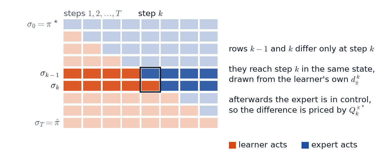
Step 1: where the two runs meet. $\sigma_k$ and $\sigma_{k-1}$ both let the learner act for the first $k-1$ steps, so they reach step $k$ in the same state, drawn from the learner’s own distribution $d^k_{\hat\pi}$.
Step 2: what differs. At step $k$, $\sigma_k$ lets the learner act while $\sigma_{k-1}$ lets the expert act, and afterwards both hand control to the expert. If the two actions agree, nothing differs. If they disagree, the difference is at most $\kappa_k$. The learner’s later mistakes are not part of this price; they are counted in later terms of the sum, at the states where they happen.
Step 3: add over the steps. With $\tilde\epsilon_t$ the probability that the learner disagrees with the expert at step $t$ on its own states,
\[\boxed{ J(\hat\pi)-J(\pi^\star)\leq\sum_{t=1}^{T}\kappa_t\,\tilde\epsilon_t, \qquad \tilde\epsilon_t=\mathbb{E}_{x\sim d^t_{\hat\pi},\,\hat u\sim\hat\pi(x)}\big[\mathbf{1}\{\hat u\neq\pi^\star(x)\}\big] }.\]If no mistake costs more than a constant $K$, this is at most $K\sum_t\tilde\epsilon_t$, which is linear in the horizon. If a mistake at step $t$ can cost the whole remaining episode, then $\kappa_t=T-t+1$ and the quadratic behavior returns.
But look at where the mistakes are counted. $\tilde\epsilon_t$ is the disagreement rate on the learner’s own states, while behavior cloning only controls $\epsilon_t$, the rate on the expert’s states. A forgiving expert is no help to a learner that was never shown how to recover: after its first mistake, the learner, not the expert, stays in control, in states it never trained on. Ross and Bagnell (2010) point out that even in forgiving tasks like these, behavior cloning can still pay a cost quadratic in $T$.
Their fix, forward training, trains each step on the right distribution. It learns a separate policy for every timestep, in order: the policy for step $t$ is trained on the states reached by running the already-trained policies for steps $1$ through $t-1$, labeled by the expert. Its error is then measured exactly where the relay needs it, and the resulting non-stationary policy $\hat\pi_{1:T}$ satisfies
\[\boxed{ J(\hat\pi_{1:T})\leq J(\pi^\star)+\sum_{t=1}^{T}\epsilon_t\kappa_t },\]where $\epsilon_t$ is now the step-$t$ policy’s error on the states it was trained on. With the numbers from before, $T=1000$ and $\epsilon=0.001$, a task in which no mistake costs more than $K=5$ steps’ worth gives a bound of $5$ instead of $1000$.
Takeaway. Recoverability attacks the second factor of $T$: in a forgiving task, a mistake costs a bounded amount, and the gap can grow only linearly with the horizon. But the mistakes have to be counted on the learner’s own states, so the learner has to be trained there. An expert’s ability to recover is no help to a behavior-cloned learner that has never seen where its mistakes lead.
Training where the learner goes: DAgger
Forward training works, but it needs a separate policy for every timestep and $T$ rounds of data collection. Its lesson is the one to keep: the error that matters is the error on the learner’s own states. Can a single policy be trained on the states it actually visits?
DAgger, short for Dataset Aggregation (Ross et al., 2011), does this in rounds. Each round rolls out a mixture of the expert and the current learner,
\[\pi_i=\beta_i\pi^\star+(1-\beta_i)\hat\pi_i,\]which means that at each step the expert acts with probability $\beta_i$ and the learner acts otherwise. Round $i$ then has four steps:
- Roll out $\pi_i$ and record the states it visits.
- Ask the expert which action it would have taken at each of those states.
- Add these state-action pairs to the dataset.
- Retrain the learner on everything collected so far.
Early rounds lean on the expert (large $\beta_i$), so rollouts stay near sensible states. As $\beta_i$ shrinks, more of the data comes from the learner’s own drift, labeled with the expert’s corrections. For the reaching arm, picture a teleoperator watching the robot wander and saying, at each pose it wanders into, which way to go from there.
To state the guarantee, let $\ell(x,\pi)$ be the training loss of policy $\pi$ at state $x$, and let \(\ell_i(\pi)=\mathbb{E}_{x\sim d_{\pi_i}}[\ell(x,\pi)]\) be its average over the states collected in round $i$. The best single policy in the class $\Pi$, chosen in hindsight, has average loss
\[\boxed{ \epsilon_N=\min_{\pi\in\Pi}\frac{1}{N}\sum_{i=1}^{N}\ell_i(\pi) }.\]If the online learner used by DAgger has vanishing average regret, its average loss approaches this hindsight benchmark. Under the theorem’s assumptions and with $N=\widetilde{O}(T)$ rounds, this gives a guarantee on the learner’s own states:
\[\boxed{ \mathbb{E}_{x\sim d_{\hat\pi}}[\ell(x,\hat\pi)]\leq\epsilon_N+O(1/T) }.\]When the loss upper-bounds the zero-one disagreement and every $\kappa_t$ is at most $\kappa$, the corresponding performance bound is
\[\boxed{ J(\hat\pi)\leq J(\pi^\star)+\kappa T\epsilon_N+O(1) }.\]This is the relay bound from the previous section, now for a single policy. $\epsilon_N$ controls the disagreement rate on the learner’s own states, which is exactly where the relay counts mistakes, and $\kappa$ prices each of them.
In finite samples, the guarantee on the learner’s states separates four sources of error:
\[\begin{aligned} \text{loss on learner states}\;\leq\;&\underbrace{\hat\epsilon_N}_{\text{empirical training loss}} +\underbrace{\gamma_N}_{\text{online-learning regret}}\\ &+\underbrace{\Delta_{\mathrm{mix}}(\beta_{1:N})}_{\text{expert-mixing schedule}} +\underbrace{\Delta_{\mathrm{sample}}(m)}_{\text{finite rollout data}}. \end{aligned}\]DAgger is not free. It needs an expert who can label arbitrary states on demand, and an environment in which an imperfect learner can be rolled out.
Takeaway. DAgger changes the guarantee from small error on the expert’s states to small error on the learner’s states. It fixes distribution shift at the source instead of assuming it away, at the price of an interactive expert and learner rollouts.
Changing the loss: log-loss and the horizon
Forward training and DAgger both need an interactive expert. Without one, it is tempting to conclude that the quadratic penalty is simply the price of learning offline. But the $T^2\epsilon$ analysis also made a choice: it scored errors with the zero-one loss, one step at a time. If we train with a different loss, does the horizon dependence change?
With discrete actions, it does (Foster et al., 2024). Training with logarithmic loss, that is, maximum likelihood on the demonstrated actions, gives a guarantee on whole trajectories. To keep costs and rewards distinct, write $V(\pi)$ for expected cumulative reward, with larger values preferred. For a deterministic expert,
\[V(\pi^\star)-V(\hat\pi)\leq 4R\,D_H^2(P_{\hat\pi},P_{\pi^\star}),\]where $R$ is the range of cumulative reward and $D_H^2$ is the squared Hellinger distance between the learner’s and the expert’s trajectory distributions. For a finite policy class trained on $n$ demonstrations, with probability at least $1-\delta$,
\[\boxed{ V(\pi^\star)-V(\hat\pi)\leq 8R\,\frac{\log(2|\Pi|/\delta)}{n} }.\]For a stochastic expert, the guarantee also depends on how much the expert’s value varies:
\[V(\pi^\star)-V(\hat\pi) \leq \sqrt{6\sigma_\star^2D_H^2} +O\!\left(R\log\frac{R}{\eta}\right)D_H^2+\eta,\]where $\eta>0$ is a tolerance and $\sigma_\star^2$ compares the expert’s value $V_t^\star(x_t)$ with its action-value $Q_t^\star(x_t,u_t)$, both measured in reward:
\[\sigma_\star^2=\sum_{t=1}^{T}\mathbb{E}\left[(V_t^\star(x_t)-Q_t^\star(x_t,u_t))^2\right].\]The finite-class bound has no explicit $T$. The horizon can enter only through $R$, the range of total reward. With a success-or-failure reward, $R=1$ and the bound does not depend on the horizon at all. With per-step rewards in $[0,1]$, $R\leq T$ and the bound is linear in $T$, not quadratic.
Why does the loss matter so much? The zero-one analysis looks at the learner one step at a time and then asks how the steps compound. Log-loss scores each demonstration as a whole. The likelihood of a demonstrated trajectory under the learner is the product of the learner’s probabilities for each demonstrated action, since the dynamics are shared by both policies and cancel out. Maximizing that likelihood controls the distance between the learner’s and the expert’s trajectory distributions, and the learner’s distribution is the one its own rollouts produce, so the effect of its actions on its future states is already included. The rate is set by the number of demonstrations $n$, not by their length.
These guarantees rely on discrete-action ingredients. With a deterministic expert, for example, the learner must put real probability on exactly the expert’s action. They should not be carried over automatically to continuous controls, where exact agreement almost never happens.
Takeaway. The $T^2$ penalty is not a law of offline imitation. With discrete actions, log-loss matches whole trajectories, and the explicit horizon factor disappears.
When mistakes stay small
So far, a mistake has been all-or-nothing: the learner either matched the expert’s action or it did not, and we asked how bad things could get afterwards. Now turn the question around. What property of the system keeps the amplification factor small, and how does the size of an action error enter? To answer this, we first make the $Q$-function picture exact.
We used a relay in the recoverability section, with the learner running first. Now run it the other way round. Let $\pi^{(k)}$ be the policy that follows the expert for the first $k$ steps and then hands control to the learner for the rest of the episode. Then $\pi^{(0)}$ is the learner and $\pi^{(T)}$ is the expert, so the deployment gap is a telescoping sum:
\[J(\hat\pi)-J(\pi^\star)=J(\pi^{(0)})-J(\pi^{(T)})=\sum_{k=1}^{T}\Big[J(\pi^{(k-1)})-J(\pi^{(k)})\Big].\]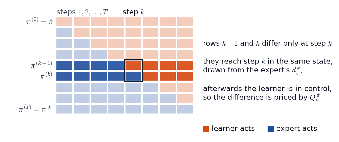
Look at one term. The policies $\pi^{(k-1)}$ and $\pi^{(k)}$ both follow the expert for the first $k-1$ steps, so they pay the same cost there and arrive at step $k$ in the same state, drawn from $d^k_{\pi^\star}$. Both also leave the learner in control from step $k+1$ onward. They differ in exactly one decision: at step $k$, $\pi^{(k-1)}$ lets the learner act, while $\pi^{(k)}$ lets the expert act. That difference is the price of one wrong action:
\[J(\pi^{(k-1)})-J(\pi^{(k)}) =\mathbb{E}_{x_k\sim d^k_{\pi^\star}}\,\mathbb{E}_{\hat u_k\sim\hat\pi(x_k)}\Big[Q_k^{\hat\pi}(x_k,\hat u_k)-Q_k^{\hat\pi}(x_k,u_k^\star)\Big].\]Summing over $k$ gives an exact identity for the deployment gap, a finite-horizon form of the performance difference lemma of Kakade and Langford (2002):
\[\boxed{ J(\hat\pi)-J(\pi^\star) =\sum_{t=1}^{T}\mathbb{E}_{x_t\sim d^t_{\pi^\star}}\,\mathbb{E}_{\hat u_t\sim\hat\pi(x_t)}\Big[Q_t^{\hat\pi}(x_t,\hat u_t)-Q_t^{\hat\pi}(x_t,u_t^\star)\Big] }.\]The details of this identity answer questions that may have looked arbitrary earlier. The states come from the expert’s distribution because the expert was in control before the hand-over, which is why errors measured on demonstrations appear at all. The $Q$-function is the learner’s because the learner lives with the consequences after the hand-over. And each term prices exactly one swapped action. Every bound in this section comes from bounding the bracket.
Smooth $Q$. Suppose $Q$ is $L$-Lipschitz in the action:
\[\boxed{\lvert Q_t^{\hat\pi}(x,u)-Q_t^{\hat\pi}(x,u')\rvert\leq L\|u-u'\|}.\]Then each bracket is at most $L\lVert\hat u_t-u_t^\star\rVert$, and summing gives
\[\boxed{J(\hat\pi)-J(\pi^\star)\leq L\,R_{\mathrm{expert},L_1}(\hat\pi)}.\]The amplification factor is now $L$, which measures how sensitive the future cost is to the action, and it contains no $T$. The training error still sums over $T$ steps: a learner that is off by $\epsilon$ at every step has $R_{\mathrm{expert},L_1}=T\epsilon$, so the gap is linear in $T$. With $T$ chances to err, each costing something, that is the best we can hope for.
Bounded $Q$. If we cannot prove smoothness but know that $0\leq Q_t^{\hat\pi}(x,u)\leq B$, then each bracket is at most $B$ when the actions differ and zero when they agree:
\[\boxed{J(\hat\pi)-J(\pi^\star)\leq B\,R_{0,1}(\hat\pi)}.\]This gives a useful sanity check. $Q_t$ can never exceed the remaining horizon, so $B=T$ always works, and then $J(\hat\pi)-J(\pi^\star)\leq T\,R_{0,1}\leq T\cdot T\epsilon$. That is the compounding-error bound, recovered in one line: $T^2\epsilon$ is the bounded-$Q$ bound with the only $B$ we get for free. Both of these bounds appear in Simchowitz et al. (2025).
Of the two conditions, the Lipschitz one suits robots better. Bounded $Q$ still counts disagreements with the zero-one loss and inherits that loss’s problems with continuous actions, while the Lipschitz route measures the size of each error. But it leaves a question open: where would a Lipschitz $Q$ come from?
Takeaway. The deployment gap is exactly a sum, along the expert’s trajectory, of the prices of single swapped actions. If that price grows in proportion to the size of the swap (a Lipschitz $Q$), the amplification factor is a constant and the horizon drops out of it.
Where smoothness comes from: stability
Assuming $Q$ is Lipschitz is convenient, but $Q$ summarizes the entire future of the system, so its smoothness has to come from somewhere. The natural place to look is the dynamics. If the robot’s motion damps out small disturbances, one wrong action should leave only a fading trace. Can we turn “the system forgets disturbances” into a value for $L$?
Incremental stability makes “forgets disturbances” precise. A system is exponentially incrementally input-to-state stable, or $(C,\rho)$-E-IISS (Simchowitz et al., 2025), when any two of its trajectories satisfy
\[\boxed{ \|x_{t+1}-x'_{t+1}\| \leq C\rho^t\|x_1-x'_1\| +\sum_{k=1}^{t}C\rho^{t-k}\|u_k-u'_k\| }\]for some constants $C\geq1$ and $0\leq\rho<1$. The first term says that a difference in initial states decays. The sum says that an input difference at step $k$ still matters at step $t+1$, but scaled by $\rho^{t-k}$, which shrinks the older the difference is.
Stability can come from two places. Open-loop stability is a property of the plant alone, while closed-loop stability is a property of the plant together with the policy’s feedback. A quadrotor, for example, is unstable without feedback but stable under a good controller. What matters here is the loop the learner actually runs: the plant under the learner’s feedback, where the inputs $u_k$ are pushes added on top of the learner’s actions.
Let’s follow one wrong action through such a loop. At step $t$ the learner takes $\hat u$ where the expert would take $u^\star$, which is a one-time push of size $\delta=\lVert\hat u-u^\star\rVert$. Afterwards both runs continue under the learner, with no further pushes. We need three assumptions:
- the learner’s closed loop is $(C,\rho)$-E-IISS;
- the learner is $L_{\hat\pi}$-Lipschitz in the state;
- the per-step cost is $1$-Lipschitz in the state and the action.
In symbols, the last two say
\[\begin{aligned} \|\hat\pi(x)-\hat\pi(x')\|&\leq L_{\hat\pi}\|x-x'\|,\\ \lvert c_t(x,u)-c_t(x',u')\rvert&\leq\|x-x'\|+\|u-u'\|. \end{aligned}\]Step 1: the state differences decay geometrically. Applying the definition with a single push,
\[\|\Delta x_{t+1}\|\leq C\delta,\qquad \|\Delta x_{t+2}\|\leq C\rho\,\delta,\qquad \|\Delta x_{t+3}\|\leq C\rho^2\delta,\qquad\ldots\]Step 2: their total is a geometric series. Because $0\leq\rho<1$,
\[\sum_{j\geq1}\|\Delta x_{t+j}\|\leq C\delta\,(1+\rho+\rho^2+\cdots)=\frac{C}{1-\rho}\,\delta.\]Step 3: convert state differences into cost differences. Three kinds of terms make up $Q_t^{\hat\pi}(x,\hat u)-Q_t^{\hat\pi}(x,u^\star)$:
- the pushed action itself at step $t$, which changes that step’s cost by at most $\delta$;
- the state differences at later steps, which add at most $\frac{C}{1-\rho}\delta$ in total;
- the action differences at later steps, which appear because the learner reacts to the shifted states. Each is at most $L_{\hat\pi}$ times the state difference, so together they add at most $L_{\hat\pi}\frac{C}{1-\rho}\delta$.
Adding the three, and using $C\geq1$ and $\frac{1}{1-\rho}\geq1$ to absorb the first term,
\[\lvert Q_t^{\hat\pi}(x,\hat u)-Q_t^{\hat\pi}(x,u^\star)\rvert \leq\delta+(1+L_{\hat\pi})\frac{C}{1-\rho}\,\delta \leq\frac{C}{1-\rho}(2+L_{\hat\pi})\,\delta.\]So $Q$ is Lipschitz with constant
\[\boxed{L_Q=\frac{C}{1-\rho}(2+L_{\hat\pi})},\]and the result of the previous section gives
\[\boxed{ J(\hat\pi)-J(\pi^\star) \leq \frac{C}{1-\rho}(2+L_{\hat\pi})\,R_{\mathrm{expert},L_1}(\hat\pi) }.\]This is Lemma 2.1 of Simchowitz et al. (2025). Each piece of the constant has a meaning. The factor $\frac{1}{1-\rho}$ is how long a disturbance lingers, and $C$ allows for a transient overshoot before the decay sets in. The $2$ counts the direct effect of the wrong action and the state drift it causes. And $L_{\hat\pi}$ says that the learner’s own sensitivity matters: a policy that reacts sharply to small state changes turns a small drift into large action differences.
The geometric series is the heart of the argument, so it is worth seeing what happens as $\rho$ crosses $1$. The interactive figure below follows one push and adds up its effect over an episode of $T$ steps.
Move ρ across 1. The blue curve adds the orange contributions as time advances.
Scalar example: a unit disturbance contributes ρʲ at lag j, with C = 1. The plot sums j = 0 through T − 1. Only ρ < 1 gives the finite infinite-horizon bound 1/(1 − ρ).

For $T=100$, the accumulated effect is about $10$ when $\rho=0.9$ (and never more, however long the episode), exactly $100$ when $\rho=1$, and about $1.4\times10^5$ when $\rho=1.1$. Contracting dynamics give a constant amplification, marginal dynamics give $O(T)$, and expanding dynamics give amplification exponential in the horizon. This is the same funnel picture as in the action chunking stability project page.
Takeaway. Stability turns a horizon-dependent amplification into a geometric series, $C+C\rho+C\rho^2+\cdots=C/(1-\rho)$. When the learner’s closed loop forgets disturbances, a small action error has a bounded total effect however long the task is. Note that the assumption is about the learner’s loop, not the expert’s.
Robots have continuous actions
Most of the results so far were built on counting disagreements: did the learner choose exactly the expert’s action? For a robot choosing among a few discrete options, that is a natural question. A robot arm, though, sends real-valued commands: torques, joint velocities, end-effector twists. What happens to exact matching when actions are real numbers?
A one-dimensional example settles it (Proposition 2.3 of Simchowitz et al., 2025). Take the class of $1$-Lipschitz functions
\[\mathcal{G}=\{g:[0,1]\to[-1,1]\text{ that are 1-Lipschitz}\},\qquad z\sim\mathrm{Unif}[0,1],\]and think of $z$ as the state and $g(z)$ as the expert’s action. However many samples $n$ the learner sees, the minimax risk under exact matching, which is the best achievable worst-case probability of missing the exact value, stays at $1$:
\[\boxed{ \forall n\in\mathbb{N},\qquad \inf_{\hat g}\sup_{g^\star\in\mathcal{G}} \mathbb{E}\left[\mathbf{1}\{\hat g(z)\neq g^\star(z)\}\right]=1 }.\]Yet the squared error shrinks at the usual rate:
\[\boxed{ \inf_{\hat g}\sup_{g^\star\in\mathcal{G}} \mathbb{E}\left[(\hat g(z)-g^\star(z))^2\right]\lesssim\frac{1}{n} }.\]There is no contradiction here. If the expert commands $0.53721$ and the learner commands $0.53720$, squared error calls the prediction nearly perfect, while exact matching calls it a miss. From finitely many samples, no learner can pin down a real-valued function exactly at every point, so under the zero-one loss essentially every prediction is a miss.
In terms of the earlier bounds, essentially every step now counts as a mistake, so $R_{0,1}\approx T$, and the bounds built on counting mistakes lose their force. The compounding-error bound, for instance, becomes $T^2$, more than the largest possible cost. The Lipschitz and stability results, which measure the size of each error, are the ones that survive.
Takeaway. For continuous actions, the right question is “how close?”, not “exactly equal?”. That moves us to norm-based errors, and a small norm error is only as good as the system’s sensitivity to it.
A small gain error, an unstable robot
The stability result gave a clean guarantee, but look again at its assumption: the learner’s closed loop must forget disturbances. That is an assumption about the learner, and the learner is exactly what we are unsure of. Can a policy have a small training error and still close an unstable loop? A one-dimensional example shows how it can.
Consider a scalar linear system
\[\boxed{x_{t+1}=ax_t+bu_t},\]and think of $x_t$ as the tilt of a balancing robot. The expert uses linear feedback $u_t=-k^\star x_t$, so its closed loop is
\[x_{t+1}=(a-bk^\star)x_t=\rho\,x_t,\qquad \lvert\rho\rvert<1.\]Normalize the initial tilt to $x_1=1$. The expert’s tilt then decays as $\lvert x_t\rvert=\lvert\rho\rvert^{t-1}$. The learner also uses linear feedback, $\hat u_t=-\hat k x_t$, with gain error $\Delta k=\hat k-k^\star$.
Step 1: the error at each expert state. On the expert’s trajectory, the learner’s action error is
\[\lvert\hat u_t-u_t^\star\rvert=\lvert\hat k-k^\star\rvert\,\lvert x_t\rvert=\lvert\Delta k\rvert\,\lvert\rho\rvert^{t-1}.\]Step 2: average over the demonstration. The horizon-averaged action error, which is $R_{\mathrm{expert},L_1}/T$ in our earlier notation, is a geometric sum:
\[R_{\mathrm{train}} =\frac{\lvert\Delta k\rvert}{T}\sum_{j=0}^{T-1}\lvert\rho\rvert^j =\frac{\lvert\Delta k\rvert}{T}\,\frac{1-\lvert\rho\rvert^T}{1-\lvert\rho\rvert}.\]For fixed $\lvert\rho\rvert<1$ and large $T$,
\[\boxed{R_{\mathrm{train}}\approx\frac{\lvert\Delta k\rvert}{T(1-\lvert\rho\rvert)}}.\]Step 3: deploy the learner. Under its own feedback, the learner’s tilt evolves as $x_{t+1}=(a-b\hat k)x_t$, so its closed-loop multiplier is
\[\boxed{\rho'=a-b\hat k=\rho-b\,\Delta k}.\]If \(\lvert\rho'\rvert>1\), the learner’s tilt grows like \(\lvert\rho'\rvert^{t-1}\), which is exponential.
Now put in numbers. Take a toy robot whose tilt doubles every step when left alone, $a=2$, with $b=1$. The expert uses $k^\star=1.05$, so $\rho=0.95$: each step, its feedback removes 5% of the tilt. Suppose the learner ends up with $\hat k=0.95$, so $\Delta k=-0.1$. At every demonstrated state, its action is within 10% of the expert’s, and over a $T=100$ step demonstration its average action error is
\[R_{\mathrm{train}}\approx\frac{0.1}{100\times0.05}=0.02.\]But its own loop has \(\rho'=0.95+0.1=1.05\): each step, it adds 5% to the tilt. After 100 steps, the expert’s tilt is down to 0.6% of where it started, and the learner’s is 125 times larger. The interactive figure below lets you compare the expert with different learner gains.
Compare k = 0.95 and k = 1.15. Both differ from the expert by 0.10, but their rollouts go in opposite directions.
Exact scalar model: xₜ₊₁ = 2xₜ + uₜ, uₜ = −kxₜ, x₁ = 1. The expert uses k = 1.05. The vertical axis is logarithmic; the readout averages absolute action error over the first T expert states. This is a worked example, not the general lower-bound construction.

Why doesn’t the training error notice? Look at where it comes from: $\lvert\Delta k\rvert\,\lvert x_t\rvert$. The figure reports its average over the demonstration. The expert’s tilt shrinks geometrically, so after the first few dozen steps the demonstration shows a robot sitting almost upright and commanding almost nothing, and every gain predicts almost nothing there. The first $1/(1-\lvert\rho\rvert)=20$ steps carry about two thirds of the total error, and averaging over $T$ steps dilutes that information by $1/T$. With a $T=1000$ step demonstration, the same wrong gain has $R_{\mathrm{train}}\approx0.002$, ten times smaller, while the learner’s rollout only gets worse.
The sign of the error matters too. With $\Delta k=+0.1$ instead (set the slider to $1.15$), \(\rho'=0.85\) and the learner is more stable than the expert. Both learners have exactly the same training error, because $R_{\mathrm{train}}$ depends only on $\lvert\Delta k\rvert$. One balances better than the expert, and the other falls over. The training error cannot tell them apart.
Takeaway. A stable expert’s demonstrations contract toward equilibrium, where every policy looks alike. A learner can match them closely and still close its loop with the wrong gain, because the quantity that decides stability, \(\rho'=\rho-b\,\Delta k\), barely shows up in the data.
How bad can it get? The lower bounds
One scalar example shows a mechanism, not a law. Maybe a smarter algorithm or a better policy class would avoid it. Is there any learner that always turns small demonstration error into small deployment error when actions are continuous? The lower bounds of Simchowitz et al. (2025) say no, in a precise worst-case sense.
The headline statement is that for some clipped-cost problems, rollout error can exceed expert-state $L_2$ imitation error by a factor exponential in the horizon:
\[\boxed{ \text{worst-case }R_{\mathrm{cost}} \geq e^{\Omega(T)}\times \text{worst-case }R_{\mathrm{expert},L_2} }.\]This is a minimax statement over constructed families of problems. It is not a forecast for every robot. It says that low demonstration error alone cannot rule out severe deployment error across the whole class of problems considered.
A more detailed version (their Theorem 1) makes the rates explicit. Let $\bar\epsilon_n=n^{-s/k}$, with $s\geq2$ and state dimension $d=k+2$. There is a family of incrementally stable instances on which a learner achieves
\[\boxed{\mathbb{E}\,R_{\mathrm{expert},L_2}\leq C_1\bar\epsilon_n}\]for every instance, while every learner in a specified class of smooth Markov policies, which act on the current state alone, faces some instance with
\[\boxed{ \mathbb{E}\,R_{\mathrm{cost}} \geq C_2\min\left\{1.05^T\bar\epsilon_n,\frac{1}{ML^2}\right\} }.\]Here $C_1,C_2,M,L$ are the constants and problem parameters of the construction (this $L$ is not the Lipschitz constant of $Q$ from earlier). Read it as a game. Nature picks an instance from the family; the learner sees $n$ demonstrations and outputs a policy. On every instance, the demonstration error can be driven down at the usual nonparametric rate $\bar\epsilon_n$. But for every learner in the class, some instance makes the rollout cost larger by a factor that grows like $1.05^T$, until it saturates at $1/(ML^2)$. That factor is the same kind of growth our toy learner showed: a loop that multiplies deviations by a little more than one at every step.
The failure is not a rare event. A strengthened construction (their Theorem 2) gives
\[\boxed{ \mathbb{E}[\mathrm{cost}] \geq C_3\min\left\{1.05^T\bar\epsilon_n,L^{-2}M^{-1}\right\} \geq C_4 },\]while the expert has zero cost on these instances.
Adding noise is not, by itself, an escape. Adding state-independent noise to a smooth mean policy does not remove the lower bound: the corresponding bounds (their Theorem 3) still contain an exponential term, with extra dependence on how spread out the noise is (its anti-concentration). More informative data or richer, state-dependent randomness may change the picture, but simple randomization is not a guarantee.
Finally, consider systems that are open-loop unstable but stabilized by the expert’s feedback, like our toy robot, whose tilt doubles every step without control. For a constructed family (their Theorem 4),
\[\boxed{ \mathbb{E}\,R_{\mathrm{expert},L_2}\leq C_1\bar\epsilon_n, \qquad \mathbb{E}\,R_{\mathrm{cost}}\geq C_2\min\{2^T\bar\epsilon_n,1\} }.\]This result holds for a broad algorithm class, including nonsmooth, stochastic, and history-dependent policies, so in this setting no choice of policy representation fixes the problem. What is missing is information. The demonstrations never show how to act away from the expert’s path, and in an open-loop unstable system, small deviations push the learner away from that path.
Takeaway. The lower bounds are worst-case statements about families of problems, not forecasts for every robot. What they establish is that low demonstration error does not, by itself, pin down the feedback behavior a robot needs away from the expert’s path. The data, or the system, has to supply it.
Putting it together
We started with one question: when does a small training error imply good behavior at deployment? Every result along the way fit the same template,
\[J(\hat\pi)-J(\pi^\star)\;\lesssim\;A\times\text{training error},\]and each one either bounded the amplification factor $A$ or changed the training error itself.
| Result | Assumption | Training error | Amplification factor |
|---|---|---|---|
| Compounding error (behavior cloning) | none | $R_{0,1}\leq T\epsilon$ | $T$ |
| Recoverability (forward training) | one wrong action, then the expert, costs at most $K$ | zero-one error on the learner’s states | $K$ |
| DAgger | the same, plus an interactive expert | loss on the learner’s states, $T\epsilon_N$ | $\kappa$ |
| Log-loss | discrete actions | $D_H^2(P_{\hat\pi},P_{\pi^\star})$, of order $\log\lvert\Pi\rvert/n$ | $4R$ |
| Bounded $Q$ | $0\leq Q\leq B$ | $R_{0,1}$ | $B$ |
| Lipschitz $Q$ | $Q$ is $L$-Lipschitz in the action | $R_{\mathrm{expert},L_1}$ | $L$ |
| Incremental stability | learner’s closed loop is $(C,\rho)$-E-IISS | $R_{\mathrm{expert},L_1}$ | $\frac{C}{1-\rho}(2+L_{\hat\pi})$ |
| Continuous-action lower bounds | worst case over constructed families | $R_{\mathrm{expert},L_2}$ | $e^{\Omega(T)}$ |
When reading a new imitation-learning result, it helps to ask six questions in order:
- What is the training error: a zero-one loss, a norm, or a likelihood?
- On which states is it measured: the expert’s, the learner’s, or a mixture?
- What does one wrong action do to the future, and what bounds its price?
- What controls the amplification factor: the horizon, recoverability, a smooth $Q$, or stability? And whose closed loop does that assumption concern?
- Are the actions discrete or continuous, and does the error metric fit them?
- Which behavior do the demonstrations leave unidentified?
The whole story fits in one chain, from the training loss to the deployment cost:
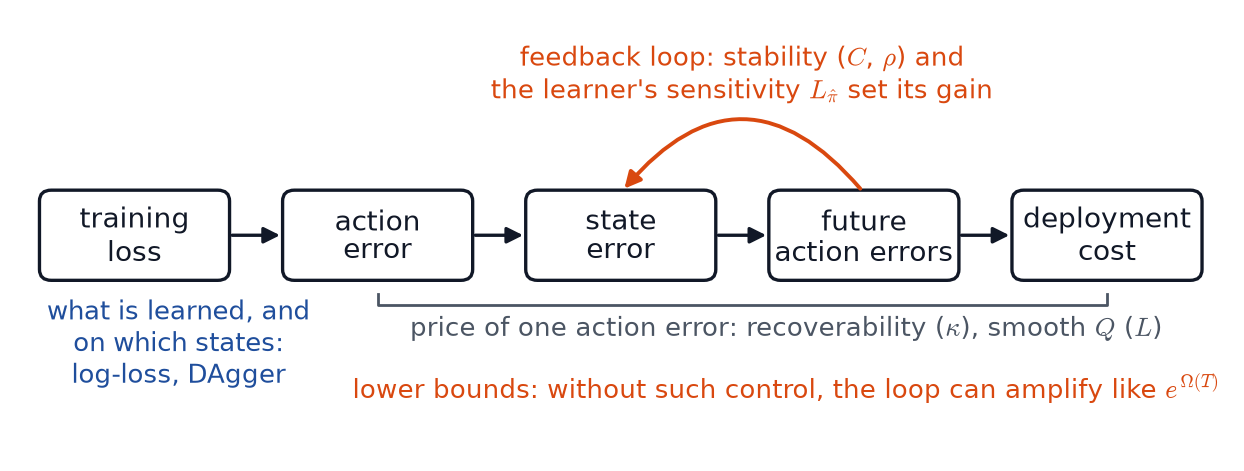
Each result controls a different part of it. The choice of loss and DAgger act on the first arrow: what the learner is trained to match, and on which states. Recoverability and a smooth $Q$ bound the whole path from one action error to its cost. Stability controls the feedback loop in the middle, where an action error moves the state and the learner’s reaction feeds back into future actions, and the lower bounds show that without such control this loop can amplify exponentially. The practical question is not simply whether the training error is small, but what the data, the loss, the policy, and the physical system together guarantee about the rollout.
References
- Foster, D. J., Block, A., and Misra, D. (2024). Is Behavior Cloning All You Need? Understanding Horizon in Imitation Learning. Advances in Neural Information Processing Systems (NeurIPS).
- Kakade, S. M., and Langford, J. (2002). Approximately Optimal Approximate Reinforcement Learning. Proceedings of the 19th International Conference on Machine Learning (ICML), 267–274.
- Ross, S., and Bagnell, J. A. (2010). Efficient Reductions for Imitation Learning. Proceedings of the 13th International Conference on Artificial Intelligence and Statistics (AISTATS), PMLR 9:661–668.
- Ross, S., Gordon, G. J., and Bagnell, J. A. (2011). A Reduction of Imitation Learning and Structured Prediction to No-Regret Online Learning. Proceedings of the 14th International Conference on Artificial Intelligence and Statistics (AISTATS).
- Simchowitz, M., Pfrommer, D., and Jadbabaie, A. (2025). The Pitfalls of Imitation Learning when Actions are Continuous. arXiv:2503.09722.